Abstract
Vibration signal contains much information about machine operational condition and has been broadly used on equipments pattern recognition. Time-frequency distribution is more suitable for nonstationary signals analysis as it provides much information both in time domain and frequency domain. A new method for machine operating condition identification is presented based on the research of Hilbert spectrum (HS) and Multi-Scale Entropy (MSE) for quantitative analysis. Firstly, HS is constructed according to the monitored signals. Then, two-dimension matrix of HS is converted to one-dimension vector. MSE can be calculated as a feature characteristic. The optimal scale will be selected by comparing MSE curves distribution for different working conditions. The sampling entropy on the selected scale and the average energy of HS are combined to construct characteristic vector. In the end, support vector machine (SVM) is used for different working conditions classification by the constructed characteristic vector. In order to verify the effectiveness of this method, experiment of different rolling bearing conditions classification is implemented in the lab. Four different operating conditions of rolling bearing can be effectively indentified by using the above method. It can be concluded that this promising method will contribute to machine condition monitoring and fault diagnosis process.
1. Introduction
With the development of production, condition monitoring and classification becomes more and more important to keep machine working in normal condition. Early fault alert and pattern recognition are essential as machines often works in off-design conditions. Incipient characteristic determination is the basis of preventative maintenance. It is also helpful for reliability estimation and remaining life prediction. There is no use for the fault diagnosis if the component is almost failure. Accurate pattern recognition can contribute to the preventative maintenance development. Different methods have been used on pattern recognition based on vibration signal analysis, such as time, frequency, resonance demodulation, and so on. As well, intelligent diagnosis and maintenance technologies have been investigated in detail for keep manufacture process [1]. Vibration signal analysis has been popularly used on machine fault diagnosis and pattern recognition, such as principal component analysis, independent component analysis, synchronous averaging technique for vibration signal analysis [2], and kurtogram for rolling element bearing (REB) fault classification [3]. Automatic feature extraction technology is also investigated on machine diagnosis [4]. At the same time, experimental investigation is beneficial for machine fault analysis [5].
But for the practical vibration signals, there are full of non-stationary and nonlinear characteristics. Traditional Fourier transform is not suitable for practical application. Time-frequency distribution (TFD) has been broadly investigated and applied on machine pattern recognition, such as short time Fourier transform, Wigner-Ville distribution, Wavelet, and so on. In 1998, Huang presented a new signal time-frequency analysis method named Hilbert spectrum (HS). HS can be obtained by using empirical mode decomposition (EMD) and Hilbert transform [6]. As this method is developed from instantaneous frequency (IF), it can well describe the non-stationary characteristics of the signal in the TFD. Thus, it is suitable for nonstationary and nonlinear signal analysis. Many researchers have investigated on this method for pattern recognition. HS can provide more information about the IF. But the classification process also depends on the ability of operators. Therefore, quantitative analysis is essential for pattern recognition. Machine fault diagnosis based on TFD classification is also investigated by Wang in 1993 [7, 8]. Frequency and time information must be considered during TFD analysis. It is important for the TFD feature extraction and quantitative estimation which can improve the accuracy for pattern recognition.
Entropy is suitable for characterizing time series’ complexity. Richman put forward sampling entropy based on the improvement of approximate entropy [9], which was presented by Pincus [10]. Costa put forward the algorithm of Multi-scale Entropy (MSE), a novel method to determine time series complexity [11]. The classification method is also important for accurate conditions analysis according to the constructed characteristic vector. One-dimension matrix can be obtained based on matrix transformation and MSE can be calculated. Therefore, MSE can be also used on TFD estimation. With the development of feature extraction, information classification method is also investigated by many researchers. Xu applies hidden markov model to processing monitoring [12]. Neural networks, D-S evidence theory and majority voting techniques have been used on machine pattern classification. Vapink has introduced support vector machine (SVM) based on statistical learning theory, which is a relatively new approach on machine working conditions monitoring and pattern recognition [13]. It is a new technology for pattern recognition which is different from neural networks, evidence theory, and Bayes method. It is a useful tool for condition classification.
In this paper, a new method for machine operational condition classification is presented by using TFD analysis. MSE analysis HS and Energy are used to construct feature vector for pattern recognition based on HS. SVM is used for different working conditions classification by the constructed characteristic vector. A REB’s working condition pattern recognition is carried out to verify the effectiveness of this method. The results show that this method will contribute the development of machine pattern recognition. This paper is structured as follows. Section 2 introduces the theory of the new method. Section 3 presents REB experiment. Section 4 provides the data analysis by using this method. Concluding remarks are given in Section 5.
2. Theory and method
2.1. Multi-scale entropy
MSE has been widely used in the analysis of physiological time series, after firstly presented by Costa. Based on sampling entropy, it can be employed to describe the irregularity of series. For a time series , which is a discrete time series with a length of . Time series can be acquired through coarse-graining transformation of Equation (1):
is the time scale. The length of coarse-grained time series is . When , the coarse-grained time series is identical to the original time series. The sampling entropy for different sampling interval can be calculated as following. According to the time series of length transformed under time scale , a -dimension vector can be constructed:
For each single , the distances can be calculated between and each of the remaining vectors :
Set as a clear threshold for the matching process. For each , which meets the condition of , and define the ratio of to the total distance as:
The average of can be expressed as:
Increasing the dimension to and repeating the above steps:
The average of is as following:
When is finite, estimated sampling entropy of series with a length of can be obtained following Equation (8):
Therefore, sampling entropy for different can be obtained by repeating the above steps. The self-similarity of time series increases with the decrease of sampling entropy, while series’ complexity increases with sampling entropy. Entropy is suitable for characterizing system complexity. Based on sampling entropy, MSE has the following merits: it can be used for multi-scale analysis; sampling entropy of different signals can be analyzed on different scales [11]. The sampling entropies of various condition signals are different on different scales. Selecting entropies with big entropy difference for characteristic vector construction can be better for condition recognition.
2.2. Characteristic parameters for Hilbert spectrum
To get a meaningful Hilbert spectrum, a new signal decomposition was introduced by Huang named as empirical mode decomposition. The decomposition process can be found in reference [6]. It is different from traditional decomposition process, which is named as EMD. According to EMD, original data is decomposed to intrinsic mode components and a residual component as Equation (9):
The original signal is decomposed to several individual and nearly mono-component signals. The mono-components obtained by EMD are named as intrinsic mode functions (IMF) to which the instantaneous frequency calculation can be applied. An IMF is a function that satisfies with the following two conditions: (i) in the whole data set, the number of extrema and the number of zero crossing points must either equal or differ at most by one; (ii) at any point, the mean value of the envelope defined by the local maxima and envelope defined the local minima is zero. Data satisfied with IMF will have well-behaved Hilbert transform, from which a meaningful IF can be calculated. For every IMF , its Hilbert transform can be expressed as:
As a result, an analytic signal, is written as:
where:
is the instantaneous amplitude of , and is the instantaneous phase of . Then, the time derivative of instantaneous phase will physically represent IF of signal , as shown Equation (13):
After finding each IMF component, Equation (14) can be obtained based on Hilbert transform. It gives both the amplitude and the frequency of the real part of each component as a function of time:
Both the amplitude and the IF can be represented in a three-dimensional plot, in which the amplitude can be contoured on a time-frequency plane. The TFD of the amplitude is expressed by HS shown as Equation (15):
HS has been broadly investigated and applied on non-stationary and nonlinear signal analysis because it was developed from IF [6]. But it can’t also provide a quantitative description of machine features. Thus, it is not suitable for practical problem analysis by operators. Further feature extraction should be carried on for pattern recognition. HS of different signals have different energy distributions in the time-frequency plane, the uniformity or complexity usually reflects different machine conditions. MSE can analyze the complexity on different scales. Thus, MSE can be used for complexity analysis of HS. HS is the two-dimensional energy matrix in the time-frequency plane. There is not any clear definition for two-dimension MSE calculation. It needs to convert HS to one-dimensional vector used for MSE analysis. The first step is to divide HS into time-frequency blocks, the energy of each block is the sum of energy of time-frequency in the corresponding region. The whole energy of HS is shown in Equation (16):
Fig. 12-D Matrix of HS converted to 1-D vector

The normalized energy distribution matrix is , the element is . Then, rows of matrix are connected and converted to one dimensional vector . Transformation process is shown as Fig. 1. Thus, the two-dimension matrix can be transformed to one-dimension for analysis. MSE can be used for entropy calculation based on MSE calculation equations. It can provide a quantitative estimation for the TFD. The quantitative estimation is suitable for practical application and better for pattern recognition.
It shows that the energy of vibration signal is different from working condition, so the average energy of HS can be taken as a characteristic value to measure the machine working conditions. It can be defined as following:
is time-frequency matrix of HS, and is the matrix size. Based on above method, the characteristic vector can be constructed by using MSE and average energy for a TFD. This vector can be used on pattern recognition for machine working condition.
2.3. Support vector machine
SVM is a new pattern recognition and statistical learning method which is developed in the end of last century. It has been broadly investigated and applied on pattern recognition area since it was introduced. The basic idea of the pattern recognition with SVM is to project sampling space into a high-dimensional eigenspace. In the eigenspace, optimal separating hyper-planes (or hyper-lines) of the original sample set can be found [13]. There are two basic classifiers for SVM. One is the binary classifier. The other is the multi-class classifier. The binary support vector classifier has been broadly applied. In this research, one-against-others type of binary SVM classifier is used for analysis. The application of one-against-others is as following: if there is a case with classes for recognition, take a top-priority class from these classes as a category and the rest classes as another category, construct a two-class SVM classifier and name it SVM1; this top-priority class is excluded. Therefore, a case of classes is left. Then, take a top-priority class from those classes as a category and the rest classes as another category. A second two-class SVM classifier is needed to construct named as SVM2, and so on. Until the last two-class SVM classifier is constructed and named SVM . In this way, two-class SVM classifiers can be constructed in all for a case of classes classification. During the fault diagnosis, the most common or the most dangerous fault can be given top priority. When an unknown fault sample is to be classified by the ‘one against others’ multi-class fault diagnosis system, its feature data is input to SVM for classification shown as Fig. 2. This classification method is more suitable for practical application. Therefore, it will be used in this research for pattern recognition.
2.4. Condition classification
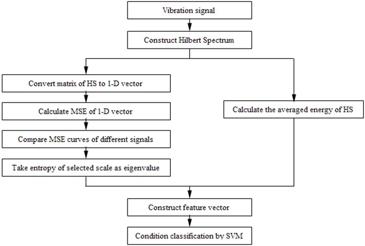
In summary, the feature extraction and working classification based on MSE for HS is as following. Firstly, the HS is constructed by the vibration signal. Then, energy matrix of HS is converted to one-dimension vector from two-dimension vector. It is convenient for quantitative analysis. By comparing MSE feature distribution of different machine condition, scale is selected. Sampling entropy of different working condition can be used to distinguish each other. Entropy of the selected scale and the averaged energy of HS are used to construct feature vector for condition classification. In the end, the vector is input to SVM for training and discrimination the working condition. The flow chart of this method is shown as Fig. 3.
Fig. 2Frame work of the one-to-others SVM algorithm
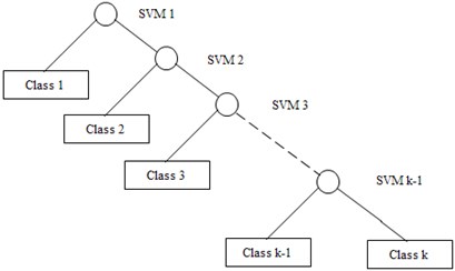
Fig. 3Flow chart for the classification process
3. Experiment
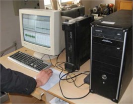
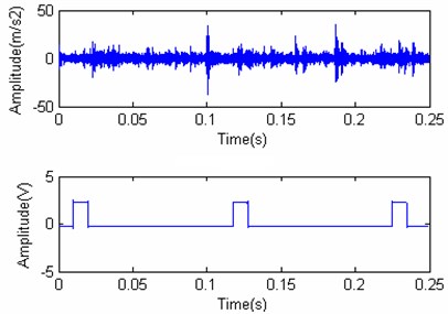
In this paper, REB conditions classification is an example to examine the effectiveness of this method in different working conditions with different speed. The type of experiment rolling bearing is N205. There are four kinds of conditions, normal working condition, ball wearing condition, inner ring wearing condition and outer ring wearing condition. Rotational velocities of the motor were 600 RPM, 900 RPM, 1200 RPM and 1500 RPM. Two acceleration sensors radical located at the bearing block were used to monitor vibration signals by BK 3560. Fig. 4 shows the pictures during the experiment in the lab. The experiment is carried on in a rolling element bearing test rig. The sampling frequency is 65536 Hz. The time domain signal with a trigger signal are shown as Fig. 5.
Fig. 4Experiment pictures in the lab
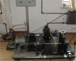
a) Test-rig
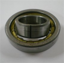
b) Inner fault
c) Data acquisition system
Fig. 5Time domain vibration signal together with trigger signal for rolling bearing
3.1. Cyclostationary signal analysis
It is also obvious that the bearing vibration signal has cyclostationary characteristics. For every working cycle, there is noise interference for the practical monitored vibration signal. The bearing vibration signal is with typical cyclostationary characteristics when it is in working condition, no matter normal or fault condition. It is very important to apply synchronous average to reduce the effect from other vibration [14, 15]. To reduce the effect from machine whole body vibration (first-order vibration) to bearing vibration signal analysis, cyclostationary model and analysis is used in this paper. Synchronous average is very useful to remove the first-order stationary effect. The second-order vibration signal can be obtained which is produced by the bearing vibration without machine body vibration after cycle average [14]. Time domain signal will be changed to angle domain signal by Spline interpolation.
Monitored vibration signal can change from time domain to angle domain by using multi-cycle synchronous average. The rotation cycle is replaced by its angle counterpart for bearing signal. Based on synchronous averaging, cyclostationary effect on signal analysis can be reduced or even removed. There are 1440 re-sampling points for every working cycle. After synchronous average, the first order vibration information can be obtained. Thus, the second order vibration signal together with noise signal can be obtained by removing first order signal. Fig. 6 shows different angle-amplitude signal for the first order vibration obtained by using synchronous average process with rotating speed in 1200 RPM without load.
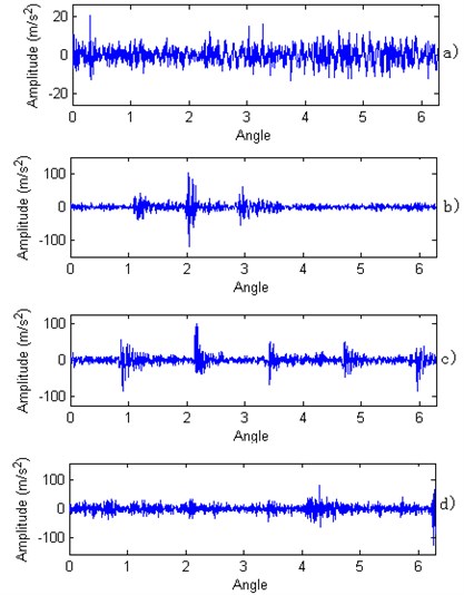
It is obvious that normal condition with small amplitude for the first order vibration signal. Compared with time domain vibration signal analysis, the impulse signal is not clear. Because the first order vibration signal is mainly related with test rig whole body vibration. On the contrary, the second order vibration signal is close related with time information for bearing vibration. For every working cycle, the second vibration signal can be obtained by removing the first order vibration signal. Fig. 7 shows second order vibration signal for different working condition with rotating speed in 1200 RPM. There is impulse information when bearing is fault condition.
Fig. 6Synchronous average for different working conditions within a working cycle. a) Normal condition; b) Inner wearing condition; c) Outer wearing condition; d) Ball wearing condition
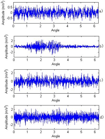
Fig. 7Second-order vibration signal for different working conditions within a working cycle. a) Normal condition; b) Inner wearing condition; c) Outer wearing condition; d) Ball wearing condition
4. Data analysis
4.1. Hilbert spectrum
REB has symmetrical structure and its vibration signal has cyclostationary characteristics. Thus, the data pre-processing can be used to improve characteristic information. Figure 8 shows different TFDs according to different working conditions vibration signals in a working cycle. Although there is difference for HS in different working conditions, it is difficult to accurately classify bearing condition just according to HS. It is similar for outer ring wearing condition and ball wearing condition by the TFD expression. At the same time, the experience of operator is important to classify machine working conditions just based on TFD without a quantitative analysis.
4.2. MSE analysis
4.2.1. MSE in time domain
MSE calculation is carried on based on time domain signals for different conditions within a working cycle. Table 1 presents the information for different working conditions. Fig. 9 provides the comparison with different working conditions. Different conditions can be classified with MSEs of time domain. It is fine for single condition classification. But MSEs don’t have the same trend with different scales shown as Fig. 10. It will have effect on pattern recognition as there is much conditions for classification in practical condition. It is the reason that time domain signal is limit to demonstrate fault characteristics.
Fig. 8Hilbert time-frequency spectrums with different working conditions
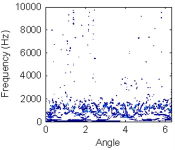
a) Normal condition
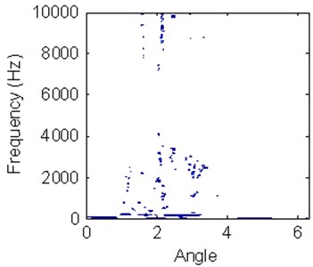
b) Inner ring wearing
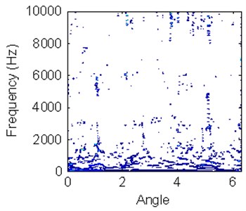
c) Outer ring wearing
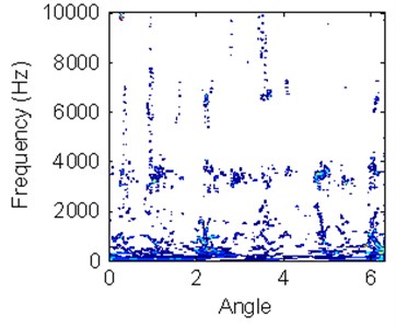
d) Ball wearing
Table 1MSE for time domain of different working conditions
Scale | 3 | 4 | 5 | 6 | 7 | 8 | 9 |
Normal condition | 1.864 | 1.881 | 1.691 | 1.889 | 1.739 | 1.631 | 1.366 |
Ball wearing | 1.3 | 1.315 | 1.182 | 1.04 | 1.011 | 0.982 | 0.915 |
Outer wearing | 0.941 | 1.049 | 0.913 | 0.834 | 0.754 | 0.668 | 0.507 |
Inner wearing | 0.847 | 0.96 | 0.99 | 0.903 | 0.938 | 0.8 | 0.748 |
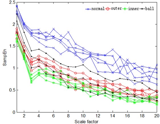
The result is shown as Fig. 11 for multi-condition classification by using MSE in time-domain signal analysis with different working conditions at speed 1200 RPM. It is difficult to classify multi-condition based on MSEs from time domain signal as they are similar for different conditions with the same scale. Only the normal condition can be distinguished from other conditions based on the scale from 3 to 9 by MSEs. MSEs for other conditions distribution of are dispersive. It is no use to classify different working condition just according to MSE for time-domain analysis as there is noise interference for practical monitored vibration signals. Time domain cannot provide much information for signal analysis and pattern recognition. The information is limit for early fault diagnosis. It is the reason that it is difficult to classify REB condition based on MSE from time domain. MSE for time domain signal is not suitable for condition classification and quantitative analysis. It also means further investigation should be carried out for feature extraction.
Fig. 9Comparison of MSEs for different scales
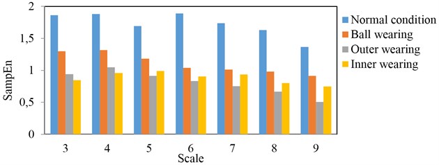
Fig. 10Relationship for different scales with different conditions classification
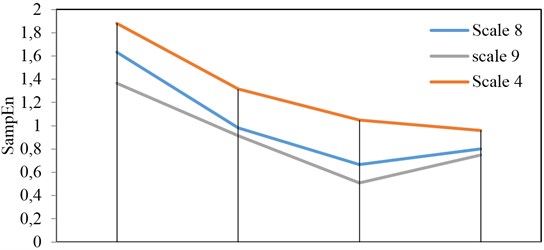
Fig. 11MSE curves of time-domain signal for different rolling bearing working condition
4.2.2. MSE of Hilbert spectrum
Based on above calculation process for MSE of HS, two-dimension matrix can be transformed to one-dimension matrix. Then, MSE can be calculated by using Equation (8). The result of MSEs for HS are present in Table 2. Figure 12 provides clearer comparison for different conditions with different scales. MSE for normal condition has the biggest value and outer wearing condition has the smallest value. MSEs for ball wearing and inner wearing are within them. Normal condition has uniform TFD in the view of time domain. According to the entropy theory, it will have the biggest entropy for the uniform distribution. There is clear impact for the inner wearing condition. Therefore, it leads to inner wearing condition is typically different with others. It also corresponds to the smallest entropy.
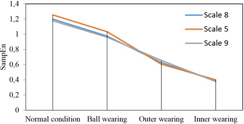
MSEs with the different conditions have the same trend for different scales. Figure 13 provides the comparison for different conditions. Curves for scale 8 and scale 9 are almost line. It has good performance on condition estimation. Curve of scale 9 is better. Therefore, it is suitable for quantitative analysis and pattern recognition. According to the results, it is easy to classify different conditions based on MSE of HS. MSE of HS is better than time-domain signal analysis based on above analysis. It can be concluded that MSE of HS can be used as a characteristic parameter to estimate machine condition.
Table 2MSE for TFD with different working conditions
Scale | 3 | 4 | 5 | 6 | 7 | 8 | 9 |
Normal condition | 1.201 | 1.247 | 1.255 | 1.23 | 1.219 | 1.2 | 1.178 |
Ball wearing | 1.023 | 1.052 | 1.035 | 1.021 | 1.01 | 0.977 | 0.961 |
Outer wearing | 0.592 | 0.593 | 0.606 | 0.612 | 0.624 | 0.628 | 0.655 |
Inner wearing | 0.415 | 0.407 | 0.401 | 0.398 | 0.39 | 0.384 | 0.378 |
Fig. 12Comparison of MSEs for different scales
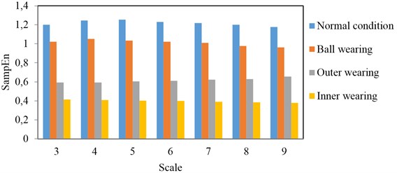
Fig. 13Relationship for different scales with different condition classification
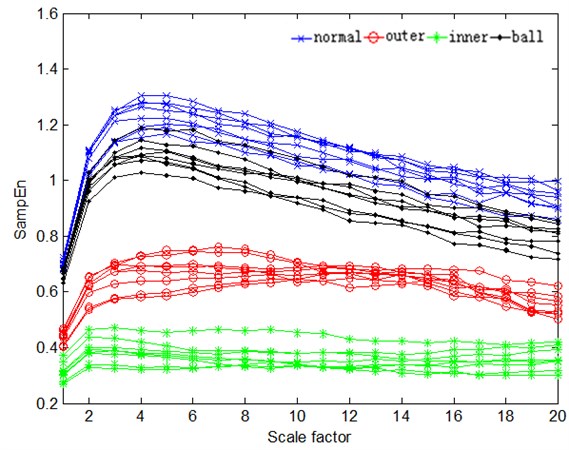
The entropy value for every condition with different scale will be broader with increasing of conditions. It increases the difficulty for pattern recognition. Figure 14 provides more MSEs curves of HS with different working conditions. Inner ring wearing and outer ring wearing are obviously distinguished from other conditions on the most scales shown as Fig. 14. But normal condition and ball wearing are a little difficult to be effectively distinguished, especially on the smaller scales. It will lead to the classification result similar for normal condition and ball wearing condition. During practical signal analysis, single parameter can not be satisfied with application as noise interference and working process complexity. More parameters can be helpful to improve the accuracy of pattern recognition. Therefore, characteristic vector can be established using MSE and other parameters to different working condition classification.
Fig. 14More condition classification based on MSE curves of HS
4.3. Classification and discussion
MSE curves of normal condition and ball wearing can’t be effectively distinguished from the Fig. 14. Other characteristic parameter can be helpful for further investigation. In practical condition, it is not suitable for classify all conditions just based on one characteristic parameter. More characteristic parameters are needed based on the machine classes. HS can be quantitatively described by the average energy of itself from the point of view of energy. The average energy can be taken as a feature value by Equation (17). Based on overall consideration, the sampling entropy with scale 9 and the average energy of HS are combined to construct characteristic vector for classification, and SVM is used for different working conditions classification. 100 samples of each working condition are selected, 50 samples for training and 50 sample for testing. Fig. 15 shows four kinds of working conditions classification result, and the result is also expressed in the Table 3. From the result, this method can effectively recognize different working conditions. It is clear in a two-dimension plane to demonstrate the different conditions.
In this research, only single fault with different conditions are used for classification. This is example to verify the effectiveness of this method on machine classification. Actually, there are many faults in machine working conditions. At the same time, several faults can happen synchronously. Therefore, one parameter is not suitable for actual problem analysis. SVM is helpful to improve the accuracy of condition classification. Multi-fault synchronous occurrence corresponds to its own TFD. TFD will present information for condition classification. Different conditions will be corresponding to different area in the SVM classification plane. Thus, multi-fault synchronous occurrence can also be classified by this method. If there are more conditions for classification, more parameters should be needed to constructed characteristic vector. Three-dimension or multi-dimension SVM classification analysis can be used. According to above analysis, it can be concluded that the method is helpful for machine condition classification based on HS feature extraction and SVM.
Fig. 15Classification result for different working condition
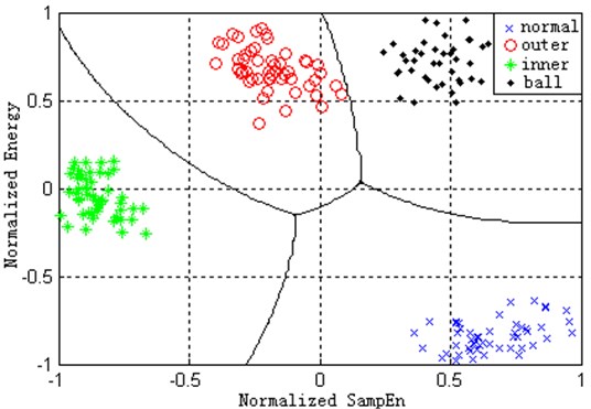
Table 3Classification result
Normal | Inner | Outer | Ball | |
Training samples | 50 | 50 | 50 | 50 |
Testing samples | 50 | 50 | 50 | 50 |
Correct samples | 50 | 50 | 50 | 50 |
Recognition rate (%) | 100 | 100 | 100 | 100 |
Total recognition rate (%) | 100 | |||
5. Conclusions
To improve the accuracy for machine condition classification, a new method is developed based on quantitative analysis of HS and SVM for pattern recognition. MSE and averaging energy can provide quantitative analysis for TFD which is beneficial for preventative maintenance. SVM is used in this research for condition classification as it is effective for small samples classification. From the example analysis of this method, it can be concluded that this new approach is effective for pattern recognition of REB. As well, this approach is also suitable to other components’ pattern recognition of machine. Thus, this promising method will contribute to machine condition monitoring and fault diagnosis process. Further research can be pursued in machine reliability estimation.
References
-
Lihovd E., Johannssen T. I., Steinebach C., Rasmussen M. Intelligent diagnosis and maintenance management. Journal of Intelligent Manufacturing, Vol. 9, Issue 6, 1998, p. 523-537.
-
McFadden P. D., Toozhy M. M. Application of synchronous averaging to vibration monitoring of rolling element bearings. Mechanical Systems and Signal Processing, Vol. 14, Issue 6, 2000, p. 891-906.
-
Eftekharnejad B., Carrasco M. R., Charnley B., Mba D. The application of spectral kurtosis on Acoustic Emission and vibrations from a defective bearing. Mechanical Systems and Signal Processing, Vol. 25, Issue 1, 2011, p. 266-284.
-
Jin J. H., Shi J. J. Automatic feature extraction of waveform signals for in-process diagnostic performance improvement. Journal of Intelligent Manufacturing, Vol. 12, Issue 3, 2001, p. 257-268.
-
Onel I. Y., Aycicek E., Senol I. An experimental study, about detection of bearing defects in inverter fed small induction motors by Concordia transform. Journal of Intelligent Manufacturing, Vol. 20, Issue 2, 2009, p. 243-247.
-
Huang N. E., Shen Z., Long S. R. The empirical mode decomposition and the Hilbert spectrum for nonlinear and non-stationary time series analysis. Proceedings of the Royal Society of London Series A-Mathematical Physical and Engineering Sciences, Vol. 454, 1998, p. 903-995.
-
Wang W. J., McFadden P. D. Early detection of gear failure by vibration analysis .1. calculation of the time-frequency distribution. Mechanical Systems and Signal Processing, Vol. 7, Issue 3, 1993, p. 193-203.
-
Wang W. J., McFadden P. D. Early detection of gear failure by vibration analysis .2. interpretation of the time-frequency distribution using image-processing techniques. Mechanical Systems and Signal Processing, Vol. 7, Issue 3, 1993, p. 205-215.
-
Richman J. S., Moorman J. R. Physiological time-series analysis using approximate entropy and sample entropy. Am. Physiological Soc., Vol. 278, Issue 6, 2000, p. 2039-2049.
-
Pincus S. M. Approximate entropy as a complexity measure. Chaos, Vol. 5, Issue 1, 1995, p. 110-117.
-
Costa M., Goldberger A. L., Peng C. K. Multi-scale entropy analysis of complex physiologic time series. Physical Review Letters, Vol. 89, 2002, p. 68-102.
-
Xu Y. S., Ge M. Hidden Markov model-based process monitoring system. Journal of Intelligent Manufacturing, Vol. 15, Issue 3, 2004, p. 337-350.
-
Vapnik V. N. The Nature of Statistical Learning Theory, Tsinghua University Press, 2000.
-
Antoni J., Daniere J., Guillet F. Effective vibration analysis of IC engines using cyclostationarity. Part I – A methodology for condition monitoring. Journal of Sound and Vibration, Vol. 257, Issue 5, 2002, p. 815-837.
-
Antoni J., Daniere J., Guillet F., Randall R. B. Effective vibration analysis of IC engines using cyclostationarity. Part II – New results on the reconstruction of the cylinder pressures. Journal of Sound and Vibration, Vol. 257, Issue 5, 2002, p. 839-856.
About this article
The work was supported by the Natural Science Foundation of China under Grant No. 51175057. The anonymous reviewers are sincerely appreciated for their valuable comments and suggestions to improve the paper.
